In this demo, we compute word-level explanations for the Huggingface textattack/roberta-base-SST-2 model, also the setup presented in the paper.

We first load required packages and the RoBERTa model. Two classes are needed to compute the explanations. BeamSearchExplainer implements the beam search algorithm, and *Masker implements the feature masking. In this demo, we use TextWordMasker since we need to mask out individual words from a text input. The other demos showcase other *Maskers.

from solvex import BeamSearchExplainer, TextWordMasker
import torch
from transformers import AutoTokenizer, AutoModelForSequenceClassification

device = 'cuda' if torch.cuda.is_available() else 'cpu'
name = 'textattack/roberta-base-SST-2'
tokenizer = AutoTokenizer.from_pretrained(name)
model = AutoModelForSequenceClassification.from_pretrained(name).to(device).eval()

The explainer expects the function to be explained in a particular format. Specifically, it takes in a list of N (full or masked) inputs, and returns a numpy array of shape N x C where C is the number of classes. The values of the array can be anything, but most commonly the class probability, which is what we are going to do here. In addition, when masking features (i.e., words) from a piece of text, TextWordMasker expects the text to be a pre-tokenized list of words and returns another list of words. Thus, sentences is a list in which each element is a list of words and the function below needs to join each sentence back to a string.

def model_func(sentences):
    sentences = [' '.join(s) for s in sentences]
    tok = tokenizer(sentences, return_tensors='pt', padding=True).to(device)
    with torch.no_grad():
        logits = model(**tok)['logits']
    probs = torch.nn.functional.softmax(logits, dim=-1).cpu().numpy()
    return probs

Now we are ready to explain! We instantiate the explainer, prepare the input sentence (as a list of words), and call the explain_instance function. The suppression argument passed to TextWordMasker tells the masker how to mask out a word. In this case, we simply delete it. The label argument to explain_instance specifies which label we want to generate the explanation for. In our case, we want to explain the positive class, which is label 1. If it is not specified, the label with the highest function value will be used.

sentence = 'A triumph , relentless and beautiful in its downbeat darkness .'.split(' ')
masker = TextWordMasker(suppression='remove')
explainer = BeamSearchExplainer(masker, f=model_func, beam_size=50, batch_size=50)
e = explainer.explain_instance(sentence, label=1)

The explanation e we get is a dictionary of keys 'exp', 'label' and 'func_val', of type list, int and float respectively, as printed out below.

print(e)
# should show: {'exp': [1.5, 8.5, 3.5, 2.5, 4.5, 9.5, 5.5, 7.5, 6.5, -0.5, 0.5], 'label': 1, 'pred': 0.9996933}

Even better, all built-in *Masker classes include more user-friendly explanation displays, and the TextWordMasker class has three. They can be called with masker.render_result, using different mode parameters. The first one is console printing.

masker.render_result(sentence, e, mode='text', execute=True)

It prints out the following texts:

Input: A triumph , relentless and beautiful in its downbeat darkness .
Explained label: 1
Function value for label 1: 1.000
Word feature attribution:
+------------+------------+
| Word       |   Attr val |
|------------+------------|
| A          |        1.5 |
| triumph    |        8.5 |
| ,          |        3.5 |
...(more rows not shown)...

The second one is color rendering.

masker.render_result(sentence, e, mode='color', execute=True)

It writes an HTML snippet to a file named explanation.html, which is rendered below.

A triumph , relentless and beautiful in its downbeat darkness . 

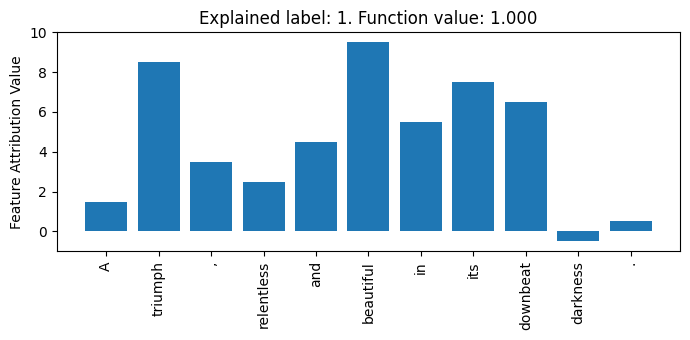
The last one is plotting.

masker.render_result(sentence, e, mode='plot', execute=True)

It generates a matplotlib figure, which is shown below.

And that's it! Want to learn more? Check out the other tabs for more use cases. If you want to gain a deeper understanding of the *Masker classes and implement your own, check out this jupyter notebook for an example where we build one from scratch and browse the documentations. Bugs? Suggestions? Questions? Ask away on GitHub!

In this demo, we compute sentence-level explanations for the Huggingface textattack/albert-base-v2-yelp-polarity model, which is designed to perform sentiment analysis on paragraph-long reviews. If you come from the previous "NLP - Word" tutorial on computing word-level explanations (no worries if not), you may have realized that this problem could be solved by manually "sentencizing" the input text and defining each "sentence" as a "word." However, in this demo, we introduce the TextSentenceMasker class which handles this sentencization automatically, using the spacy package.

We first load required packages and the ALBERT model. Two classes are needed to compute the explanations. BeamSearchExplainer implements the beam search algorithm, and *Masker implements the feature masking. In this demo, we use TextSentenceMasker since we need to mask out individual sentences from a text input. The other demos showcase other *Maskers.

from solvex import BeamSearchExplainer, TextSentenceMasker
import torch
from transformers import AutoTokenizer, AutoModelForSequenceClassification

device = 'cuda' if torch.cuda.is_available() else 'cpu'
name = 'textattack/albert-base-v2-yelp-polarity'
tokenizer = AutoTokenizer.from_pretrained(name)
model = AutoModelForSequenceClassification.from_pretrained(name).to(device).eval()

The explainer expects the function to be explained in a particular format. Specifically, it takes in a list of N (full or masked) inputs, and returns a numpy array of shape N x C where C is the number of classes. The values of the array can be anything, but most commonly the class probability, which is what we are going to do here. In addition, when masking features (i.e., sentences) from a piece of text, TextWordMasker takes the text as a string and returns another string. Thus, texts is a list of strings.

def model_func(texts):
    tok = tokenizer(texts, return_tensors='pt', padding=True).to(device)
    with torch.no_grad():
        logits = model(**tok)['logits']
    probs = torch.nn.functional.softmax(logits, dim=-1).cpu().numpy()
    return probs

Now we are ready to explain! We instantiate the explainer, prepare the input, and call the explain_instance function. When removing a sentence, TextWordMasker simply deletes it from the paragraph. The label argument to explain_instance specifies which label we want to generate the explanation for. In our case, we want to explain the positive class, which is label 1. If it is not specified, the label with the highest function value will be used.

text = ("Contrary to other reviews, I have zero complaints about "
        "the service or the prices. I have been getting tire service "
        "here for the past 5 years now, and compared to my experience "
        "with places like Pep Boys, these guys are experienced and know "
        "what they're doing. Also, this is one place that I do not feel "
        "like I am being taken advantage of, just because of my gender. "
        "Other auto mechanics have been notorious for capitalizing on "
        "my ignorance of cars, and have sucked my bank account dry. But "
        "here, my service and road coverage has all been well explained - "
        "and let up to me to decide. And they just renovated the waiting "
        "room. It looks a lot better than it did in previous years.")
masker = TextSentenceMasker()
explainer = BeamSearchExplainer(masker, f=model_func, beam_size=50, batch_size=16)
e = explainer.explain_instance(text, label=1)

The explanation e we get is a dictionary of keys 'exp', 'label' and 'func_val', of type list, int and float respectively, as printed out below.

print(e)
# should show: {'exp': [1.5, 4.5, -0.5, -1.5, 3.5, 0.5, 2.5], 'label': 1, 'func_val': 0.99981827}

Even better, all built-in *Masker classes include more user-friendly explanation displays, and the TextSentenceMasker class has three. They can be called with masker.render_result, using different mode parameters. The first one is console printing.

masker.render_result(text, e, mode='text', execute=True)

It prints out the following texts:

Explained label: 1
Function value for label 1: 1.000
Sentence feature attribution:
+--------------------------------------------------------------+------------+
| Sentence                                                     |   Attr val |
|--------------------------------------------------------------+------------|
| Contrary to other reviews, I have zero complaints about the  |        1.5 |
| service or the prices.                                       |            |
|--------------------------------------------------------------+------------|
| I have been getting tire service here for the past 5 years   |        4.5 |
| now, and compared to my experience with places like Pep      |            |
| Boys, these guys are experienced and know what they're       |            |
| doing.                                                       |            |
|--------------------------------------------------------------+------------|
| Also, this is one place that I do not feel like I am being   |       -0.5 |
| taken advantage of, just because of my gender.               |            |
............................(more rows not shown)............................

The second one is color rendering.

masker.render_result(text, e, mode='color', execute=True)

It writes an HTML snippet to a file named explanation.html, which is rendered below.

Contrary to other reviews, I have zero complaints about the service or the prices. I have been getting tire service here for the past 5 years now, and compared to my experience with places like Pep Boys, these guys are experienced and know what they're doing. Also, this is one place that I do not feel like I am being taken advantage of, just because of my gender. Other auto mechanics have been notorious for capitalizing on my ignorance of cars, and have sucked my bank account dry. But here, my service and road coverage has all been well explained - and let up to me to decide. And they just renovated the waiting room. It looks a lot better than it did in previous years. 

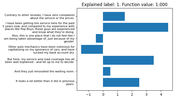
The last one is plotting.

masker.render_result(text, e, mode='plot', execute=True)

It generates a matplotlib figure, which is shown below.

And that's it! Want to learn more? Check out the other tabs for more use cases. If you want to gain a deeper understanding of the *Masker classes and implement your own, check out this jupyter notebook for an example where we build one from scratch and browse the documentations. Bugs? Suggestions? Questions? Ask away on GitHub!

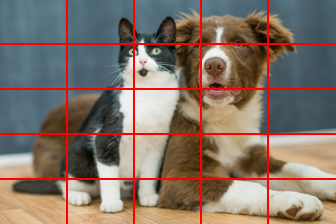
In this demo, we compute explanations for the ResNet-50 trained on ImageNet, where we define a grid of superpixels as features to perturb. The image below shows the grid superpixel segmentation. We consider each grid cell as a feature.

We first load required packages, the ResNet model and its preprocessing pipeline. Two classes are needed to compute the explanations. BeamSearchExplainer implements the beam search algorithm, and *Masker implements the feature masking. In this demo, we use ImageGridMasker since we need to mask out individual grid cells from an image input. The other demos showcase other *Maskers.

from solvex import BeamSearchExplainer, ImageGridMasker
import requests
from io import BytesIO
from PIL import Image
import numpy as np
import matplotlib.pyplot as plt
import torch
from torchvision import transforms
from torchvision.models import resnet50

device = 'cuda' if torch.cuda.is_available() else 'cpu'
model = resnet50(weights='IMAGENET1K_V2').to(device)
model.eval()
preprocess = transforms.Compose([
    transforms.ToTensor(),
    transforms.Normalize(mean=[0.485, 0.456, 0.406], std=[0.229, 0.224, 0.225]),
])

The explainer expects the function to be explained in a particular format. Specifically, it takes in a list of N (full or masked) inputs, and returns a numpy array of shape N x C where C is the number of classes. The values of the array can be anything, but most commonly the class probability, which is what we are going to do here. In addition, when masking features (i.e., pixel grids) from an image, ImageGridMasker expects the image to be a PIL.Image.Image, a numpy.ndarray or a torch.tensor object and returns another object of the same class. We choose torch.tensor so that preprocess (which is a CPU-intensive operation) is only explicitly applied once. Thus, imgs is a list of torch.tensor objects.

def model_func(imgs):
    imgs = torch.stack(imgs, dim=0)
    with torch.no_grad():
        logits = model(imgs)
    probs = torch.nn.functional.softmax(logits, dim=-1).cpu().numpy()
    return probs

Next we prepare the input image and instantiate the explainer. ImageGridMasker takes two arguments. resolution specifies the grid resolution. In our case, we want a 5 x 5 grid. It can also be a 2-tuple (r_h, r_w), for height and width resolutions. fill_value specifies the masking operation. In this case, we replace the pixel value with the average pixel value of the entire image. Other options include 'local_mean' of the grid cell and fixed pixel values in the format of an number v or a 3-tuple (r, g, b).

# download the image and resize to have shorter side length of 224 pixels
url = 'https://yilunzhou.github.io/solvability/cat_and_dog.jpg'
image = Image.open(BytesIO(requests.get(url).content))
ratio =  224 / min(image.size)
image = image.resize((np.array(image.size) * ratio).astype('int32'))
img_pt = preprocess(image).to(device)

masker = ImageGridMasker(resolution=5, fill_value='global_mean')
explainer = BeamSearchExplainer(masker, f=model_func, beam_size=50, batch_size=50)

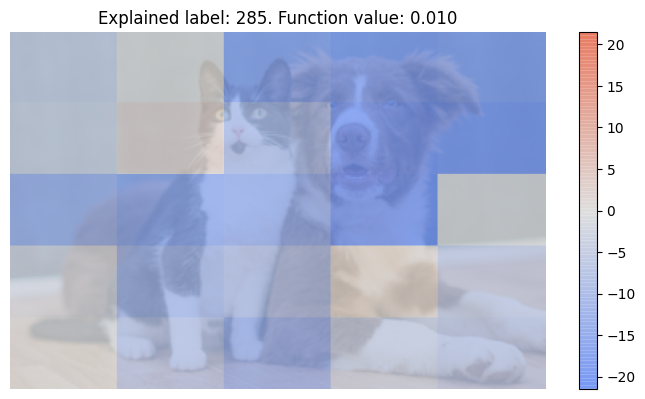
Now we are ready to explain! The image shows a dog and a cat, and we are interested in which pixels contribute the most to each label. Since there are multiple ImageNet classes for different dog and cat species, we choose the class with the highest predicted probability for each, which is class 232 (Border collie) for dog (15.9%) and class 285 (Egyptian cat) for cat (1.0%). We specify the target class via the label argument to explain_instance. If it is not provided, the label with the highest function value will be used.

e_dog = explainer.explain_instance(img_pt, label=232)  # Border collie
e_cat = explainer.explain_instance(img_pt, label=285)  # Egyptian cat

The explanation e_dog/e_cat we get is a dictionary of keys 'exp', 'label' and 'func_val', of type list, int and float respectively, as printed out below.

print(e_dog)
# should show: {'exp': [7.5, 5.5, 13.5, 17.5, 8.5, 6.5, -6.5, -5.5, 10.5, 4.5, -1.5, -4.5, -2.5, 2.5, 11.5, 9.5, 1.5, -0.5, 3.5, 14.5, 12.5, 16.5, 0.5, -3.5, 15.5], 'label': 232, 'func_val': 0.15883905}

Even better, all built-in *Masker classes include more user-friendly explanation displays, and the ImageGridMasker class has two. They can be called with masker.render_result, using different mode parameters. Note that the original PIL.Image.Image object image is passed in, needed by the color rendering mode (next one). The first one is console printing.

masker.render_result(image, e_dog, mode='text', execute=True)

It prints out the following texts:

Explained label: 232
Function value for label 232: 0.159
Grid cell feature attribution:
+------------+-----------+-----------+------------+
| Cell idx   | Row idx   | Col idx   |   Attr val |
|------------+-----------+-----------+------------|
| Cell 0     | row 0     | col 0     |        7.5 |
| Cell 1     | row 0     | col 1     |        5.5 |
| Cell 2     | row 0     | col 2     |       13.5 |
| Cell 3     | row 0     | col 3     |       17.5 |
...............(more rows not shown)...............

The second one is color overlay on top of the input image (i.e., the typical saliency map visualization).

masker.render_result(image, e_dog, mode='color', execute=True)
masker.render_result(image, e_cat, mode='color', execute=True)

Each line creates a matplotlib figure, and we show both below (dog on the left, cat on the right).

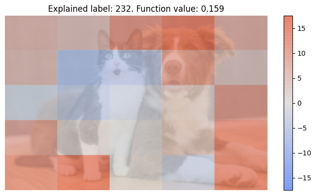
For the dog class explanation, most grid cells on the dog have very positive influence (red colors), while those on the cat face have mildly negative influence (blue colors). Curiously, the cat feet grid cell has high positive influence -- probably the model confusing them as dog feet?

For the cat class explanation, grid cells on the dog have very negative influence, meaning that their removal would significantly increase predicted probability for the cat class. By comparison, none of the features have strong positive influence. This also makes sense: we define a feature to have high positive influence if its removal greatly decreases the predicted probability, but the current probability of 1.0% is already quite low!

And that's it! Want to learn more? Check out the other tabs for more use cases. If you want to gain a deeper understanding of the *Masker classes and implement your own, check out this jupyter notebook for an example where we build one from scratch and browse the documentations. Bugs? Suggestions? Questions? Ask away on GitHub!

In this demo, we compute explanations for the ResNet-50 trained on ImageNet, where we use a custom segmentation mask to define superpixels (similar to the implementation of the LIME explanation).

We first load required packages, the ResNet model and its preprocessing pipeline. Two classes are needed to compute the explanations. BeamSearchExplainer implements the beam search algorithm, and *Masker implements the feature masking. In this demo, we use ImageSegmentationMasker since we need to mask out individual superpixels from an image input. The other demos showcase other *Maskers.

from solvex import BeamSearchExplainer, ImageSegmentationMasker
import requests
from io import BytesIO
from PIL import Image
import numpy as np
import skimage
import matplotlib.pyplot as plt
import torch
from torchvision import transforms
from torchvision.models import resnet50

device = 'cuda' if torch.cuda.is_available() else 'cpu'
model = resnet50(weights='IMAGENET1K_V2').to(device)
model.eval()
preprocess = transforms.Compose([
    transforms.ToTensor(),
    transforms.Normalize(mean=[0.485, 0.456, 0.406], std=[0.229, 0.224, 0.225]),
])

The explainer expects the function to be explained in a particular format. Specifically, it takes in a list of N (full or masked) inputs, and returns a numpy array of shape N x C where C is the number of classes. The values of the array can be anything, but most commonly the class probability, which is what we are going to do here. In addition, when masking features (i.e., superpixels) from an image, ImageSegmentationMasker expects the image to be a PIL.Image.Image, a numpy.ndarray or a torch.tensor object and returns another object of the same class. We choose torch.tensor so that preprocess (which is a CPU-intensive operation) is only explicitly applied once. Thus, imgs is a list of torch.tensor objects.

def model_func(imgs):
    imgs = torch.stack(imgs, dim=0).to(device)
    with torch.no_grad():
        logits = model(imgs)
    probs = torch.nn.functional.softmax(logits, dim=-1).cpu().numpy()
    return probs

Next we prepare the input image and instantiate the explainer. ImageSegmentationMasker takes an argument fill_value that specifies the masking operation. In this case, we replace the pixel value with the average pixel value of the entire image. Other options include 'local_mean' of the superpixel and fixed pixel values in the format of a number v or a 3-tuple (r, g, b).

# download the image and resize to have shorter side length of 224 pixels
url = 'https://yilunzhou.github.io/solvability/cat_and_dog.jpg'
image = Image.open(BytesIO(requests.get(url).content))
ratio =  224 / min(image.size)
image = image.resize((np.array(image.size) * ratio).astype('int32'))

masker = ImageSegmentationMasker(resolution=5, fill_value='global_mean')
explainer = BeamSearchExplainer(masker, f=model_func, beam_size=50, batch_size=50)

We need to define the segmentation mask for the image. A mask is a 2D integer matrix of the same height and width as the image, and values start from 0, where pixels of the same number belong to the same superpixel segment. We use the SLIC algorithm, implemented by the scikit-image package (note that the algorithm can produce fewer than the requested 40 segments; in our case, we have 29). We can visualize the mask using matplotlib.

seg_mask = skimage.segmentation.slic(image, n_segments=40, start_label=0)
plt.imshow(seg_mask)
plt.show()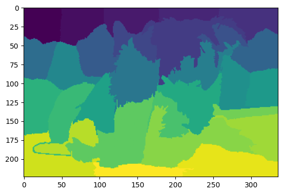

Now we are ready to explain! The image shows a dog and a cat, and we are interested in which pixels contribute the most to each label. Since there are multiple ImageNet classes for different dog and cat species, we choose the class with the highest predicted probability for each, which is class 232 (Border collie) for dog (15.9%) and class 285 (Egyptian cat) for cat (1.0%). In explain_instance, we specify the target class via the label argument, and the segmentation mask via the seg_mask argument. If label is not provided, the label with the highest function value will be used. The seg_mask argument is not a standard argument to the function, but instead "extra information" provided to the explainer, which passes all such information to ImageSegmentationMasker. For more information about how this works, see this advanced tutorial of implementing custom maskers.

e_dog = explainer.explain_instance(image, label=232, seg_mask=seg_mask)  # Border collie
e_cat = explainer.explain_instance(image, label=285, seg_mask=seg_mask)  # Egyptian cat

The explanation e_dog/e_cat we get is a dictionary of keys 'exp', 'label' and 'func_val', of type list, int and float respectively, as printed out below.

print(e_dog)
# should show: {'exp': [13.5, 6.5, 21.5, 19.5, 14.5, 25.5, -1.5, 24.5, 18.5, 1.5, 4.5, -2.5, 20.5, 3.5, 12.5, 9.5, 22.5, -0.5, 2.5, 17.5, 0.5, 23.5, 11.5, 8.5, 10.5, 15.5, 16.5, 7.5, 5.5], 'label': 232, 'func_val': 0.15883905}

Even better, all built-in *Masker classes include more user-friendly explanation displays, and the ImageSegmentationMasker class has two. They can be called with masker.render_result, using different mode parameters. Note that the original PIL.Image.Image object image is passed in, needed by the color rendering mode (next one). The first one is console printing.

masker.render_result(image, e_dog, mode='text', execute=True)

It prints out the following texts:

Explained label: 232
Function value for label 232: 0.159
Superpixel feature attribution:
+------------------+------------+
| Superpixel idx   |   Attr val |
|------------------+------------|
| Superpixel 0     |       13.5 |
| Superpixel 1     |        6.5 |
| Superpixel 2     |       21.5 |
| Superpixel 3     |       19.5 |
......(more rows not shown)......

The second one is color overlay on top of the input image (i.e., the typical saliency map visualization).

masker.render_result(image, e_dog, mode='color', execute=True, seg_mask=seg_mask)
masker.render_result(image, e_cat, mode='color', execute=True, seg_mask=seg_mask)

Each line creates a matplotlib figure, and we show both below (dog on the left, cat on the right).

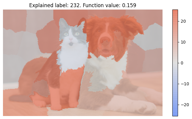
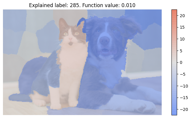
For the dog class explanation, most regions on the dog have very positive influence (red colors), while those on the cat face have mildly negative influence (blue colors). Curiously, the lower cat body regions has high positive influence -- probably the model confusing them as dog body parts?

For the cat class explanation, regions on the dog have very negative influence, meaning that their removal would significantly increase predicted probability for the cat class. By comparison, none of the features have strong positive influence. This also makes sense: we define a feature to have high positive influence if its removal greatly decreases the predicted probability, but the current probability of 1.0% is already quite low!

And that's it! Want to learn more? Check out the other tabs for more use cases. If you want to gain a deeper understanding of the *Masker classes and implement your own, check out this jupyter notebook for an example where we build one from scratch and browse the documentations. Bugs? Suggestions? Questions? Ask away on GitHub!

In this demo, we compute explanations for a random forest classifier trained on the Adult (aka Census Income) dataset. The dataset contains 14 input variables, and 1 binary target (income >50K or not). Among the 14 input variables, 13 describe demographic information, and one (fnlwgt) is final weight, or "the number of people the census believes the entry represents." Since this feature is not available at when using the model to make individual prediction, we drop it from the dataset.

We first load required packages. Two classes are needed to compute the explanations. BeamSearchExplainer implements the beam search algorithm, and *Masker implements the feature masking. In this demo, we use TabularMasker for tabular data. The other demos showcase other *Maskers.

from solvex import BeamSearchExplainer, TabularMasker
import numpy as np
import pandas as pd
from sklearn.ensemble import RandomForestClassifier
from sklearn.model_selection import train_test_split

Next, we read the dataset. The URL points to a CSV file that drops the fnlwgt feature as discussed above, but is otherwise identical to the official adult.data file. We also record the human-readable feature names and define cat_cols as a list of indices of categorical features. These features will be processed using one-hot encoding for the classifier.

D = 13  # input dimension, i.e. number of features
col_names = ['Age', 'Workclass', 'Education', 'Education-Num', 'Marital-Status', 
             'Occupation', 'Relationship', 'Race', 'Sex', 'Capital-Gain', 
             'Capital-Loss', 'Hours-per-Week', 'Native-Country']
cat_cols = set([1, 2, 4, 5, 6, 7, 8, 12])

def read_data():
    url = 'https://yilunzhou.github.io/solvability/adult.data'
    df = pd.read_csv(url, header=None, names=range(14), usecols=range(14))
    X_data = np.zeros((df.shape[0], df.shape[1] - 1))
    mappings = []
    for col_idx in range(df.shape[1] - 1):
        if col_idx in cat_cols:
            mapping = {e: i for i, e in enumerate(sorted(list(set(df[col_idx]))))}
            mapping.update({i: e for e, i in mapping.items()})
            mappings.append(mapping)
            X_data[:, col_idx] = df[col_idx].replace(mapping)
        else:
            mappings.append(None)
            X_data[:, col_idx] = df[col_idx]
    y_data = np.array(df[13].replace({'<=50K': 0, '>50K': 1}))
    return X_data, y_data, mappings

This function returns three variables. X_data and y_data are numpy arrays of shape N x D and N, where N is the number of instances, and D = 13 is the number of features. mappings is a list of D elements, one for each feature. If the feature is numerical, the element is None. If it is categorical, it is a 2-way dictionary mapping between feature names and category indices. Thus, for M categories, the dictionary has length of 2 * M.

Since the random forest classifier learns from the one-hot encoding representation, we define a wrapper on the random forest classifier to handle this automatically.

class RandomForestWrapper():
    def __init__(self, num_categories):
        self.num_categories = num_categories
    def featurize(self, X):
        arr = []
        for x in X:
            features = []
            for e, l in zip(x, self.num_categories):
                if l != -1:
                    f = np.zeros(l)
                    if e is not None: 
                        f[int(e)] = 1
                else:
                    f = np.array([e])
                features.append(f)
            arr.append(np.concatenate(features))
        arr = np.array(arr)
        return arr
    def fit(self, X, y):
        self.rf = RandomForestClassifier(random_state=0)
        return self.rf.fit(self.featurize(X), y)
    def predict_proba(self, X):
        return self.rf.predict_proba(self.featurize(X))
    def score(self, X, y):
        return self.rf.score(self.featurize(X), y)

The num_categories argument in the constructor signals numerical vs. categorical features. Specifically, it is a list of numbers, one for each feature, and a value of -1 is used to indicate a numerical feature, and otherwise a categorical feature where the value represents the number of categories. featurize takes in a list of inputs and performs the one-hot encoding. There is a special consideration in this function: it maps a None value for a categorical feature to an all zero vector to represent that none of the categories are active. Its purpose is to deal with the case where this feature is masked out by the explainer.

Now, we prepare the training and test split, train the model and evaluate it. We should obtain a training accuracy of 97.9% and a test accuracy of 84.6%.

X, y, mappings = read_data()
X_train, X_test, y_train, y_test = train_test_split(X, y, test_size=0.2, random_state=0)
num_categories = [len(m) // 2 if m is not None else -1 for m in mappings]
rf = RandomForestWrapper(num_categories)
rf.fit(X_train, y_train)
print(f'Train accuracy: {rf.score(X_train, y_train)}')
print(f'Test accuracy: {rf.score(X_test, y_test)}')

Now we are ready to explain! The explainer expects the function to be explained in a particular format. Specifically, it takes in a list of N (full or masked) inputs, and returns a numpy array of shape N x C where C is the number of classes. The values of the array can be anything, but most commonly the class probability, which is what we do here. In fact, this is the predict_proba function of our RandomForestWrapper.

In addition, TabularMasker takes one required argument, a list named suppression, one element for each feature. A value of 'cat' indicates that the feature is categorical (for which the masker replaces the feature value with None to indicate masking). For numerical features, valid values for the latter case are 'mean', 'median' and any numerical values. The first two instructs the masker to use the mean or median feature values, so we need to provide a second argument of the dataset (before one-hot encoding) for it to compute them. If it is a numerical value, it uses that value.

The label argument to explain_instance specifies which label we want to generate the explanation for. In our case, we want to explain the income less than or equal to $50K class, which is label 0. If it is not specified, the label with the highest function value will be used.

suppression = ['cat' if i in cat_cols else 'mean' for i in range(D)]
masker = TabularMasker(suppression, X_train)
explainer = BeamSearchExplainer(masker, f=rf.predict_proba, beam_size=50)

instance = X_test[0]
e = explainer.explain_instance(instance, label=0)

The explanation e we get is a dictionary of keys 'exp', 'label' and 'func_val', of type list, int and float respectively, as printed out below.

print(e)
# should show: {'exp': [8.5, 0.5, 5.5, 4.5, 6.5, -2.5, 9.5, 2.5, 7.5, 1.5, 3.5, -0.5, -1.5], 'label': 0, 'func_val': 0.98}

Even better, all built-in *Masker classes include more user-friendly explanation displays, and the TabularMasker class has two. They can be called with masker.render_result, using different mode parameters. We provide col_names and category_mappings so that the rendered results are more human-readable. The first one is console printing.

masker.render_result(instance, e, mode='text', execute=True, col_names=col_names, category_mappings=mappings)

It prints out the following texts:

Explained label: 0
Function value for label 0: 0.980
Feature attribution:
+----------------+---------------+------------+
| Feature        | Value         |   Attr val |
|----------------+---------------+------------|
| Age            | 27.0          |        8.5 |
| Workclass      | Private       |        0.5 |
| Education      | Some-college  |        5.5 |
| Education-Num  | 10.0          |        4.5 |
.............(more rows not shown).............

The second one is plotting.

masker.render_result(instance, e, mode='plot', execute=True, col_names=col_names, category_mappings=mappings)

It generates a matplotlib figure, which is shown below.

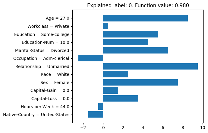
As we can see, when explaining class 0 (i.e., income less than or equal $50K), the biggest contributing (i.e., positive) factors are age (27), relationship (unmarried) and sex (female). By comparison, the administrative clerical occupation helps toward the more than $50K prediction, as does the United States as native country. In some cases, we may want the positive attribution values to indicate impact towards the "positive" label (i.e., more than $50K). We can use label=1 in explain_instance, but a more convenient thing is to add flip=True to the rendering function call.

masker.render_result(instance, e, mode='plot', execute=False, flip=True, col_names=col_names, category_mappings=mappings)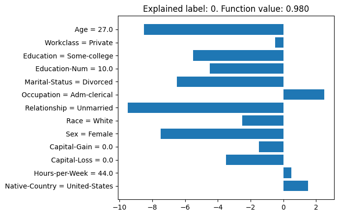

And that's it! Want to learn more? Check out the other tabs for more use cases. If you want to gain a deeper understanding of the *Masker classes and implement your own, check out this jupyter notebook for an example where we build one from scratch and browse the documentations. Bugs? Suggestions? Questions? Ask away on GitHub!