Overview [Back to Top]

This package is used to inspect and modify an ExSum rule union defined for feature attribution explanations for binary text classification models. It contains class definitions for ExSum rules and rule unions, and a Flask-based server for interactive visualization of the rules and rule unions.

Quickstart [Back to Top]

Installation

This package is available on PyPI. To install, simply run pip install exsum on the command line. Alternatively, clone the GitHub repo linked above and run pip install . inside the cloned directory.

Launching the GUI Interface

After installation, a new exsum command will be available on the command line. It should be called as

exsum model-fn [--model-var-name model --log-dir logs --save-dir saves]

The first argument model-fn specifies an exsum.Model object. It could be one of the following two:

1. a Python script (ending with .py) that defines this object in the global namespace with the default variable name being model, or
2. a Python pickle file (ending with .pkl) of that object. Note that since exsum.Model objects contain functions as instance variables (as described below), it need to be pickled by the dill library.

Steps to construct this object are detailed in the Development Manual section, but briefly, it contains the following data:

• the rule union with its constituent rules,
• the dataset on which the rule union and individual rules are evaluated, and
• the local feature attribution explanation for each instance in the dataset.

The three subsequent keyword arguments are optional.

• --model-var-name (default: model) specifies the name of the exsum.Model variable to load in the model-fn Python script. It is not applicable if a pickled object file (i.e. *.pkl) is given for model-fn.
• --log-dir argument (default: logs) specifies the logging directory. All GUI operations in an exsum session are saved as a timestamped log file to this directory.
• --save-dir argument (default: saves) specifies the location where the modified rules are saved by clicking a Save button on the GUI. Each time two files are saved, both named with the current timestamp:
  1. a plain-text file of the current parameter values of all rules, and
  2. a pickled exsum.Model object with the current parameters, which can be passed in as the model-fn parameter and loaded in a new exsum session.
  In addition, two files named latest.(txt|pkl) are also created with the same content for the user to look up easily. These files should be renamed or moved if the user wants to keep them, as they will be overwritten on the next save.

This command starts a local web server and serves the GUI continuously (i.e. will not finish unless shutdown by Ctrl-C). While it is running, open up a browser to http://localhost:5000 to interact with the GUI.
Note that this server instance is fully local. It makes no connections to other servers on the Internet (third-party CSS and JS files have been downloaded and included in the project package). Thus, the operations in the browser is only tracked by local logging to the log-dir, and not shared in any way.

Demos

To visualize the two rule unions presented in the paper, follow these steps:

0. Install exsum with pip (see above for instructions).
1. In any directory, clone the exsum-demos repository, and cd into it.

   git clone https://github.com/YilunZhou/exsum-demos
   cd exsum-demos

2. In this exsum-demo directory, run one of the two following commands to visualize the SST or QQP rule union.

   exsum sst_rule_union.py  # OR
   exsum qqp_rule_union.py

3. Open up a browser to http://localhost:5000 to interact with the GUI. Play with it, tweak things, and see what happens.

Next Steps

To better understand the GUI, continue reading the GUI Manual section for details. To study the implementation of these rule unions or write your own rules and/or rule unions, read the Development Manual section afterward.

GUI Manual [Back to Top]

The figure below shows the GUI interface with the SST rule union loaded and Rule 19 selected. Various panels are annotated.

Panel A

This panel shows the composition structure of the rules. Note that not every rule needs to be used (Rule 2 and 7 are not used here), but each rule can be used at most once.
When a rule is selected, a counterfactual (CF) rule union without this rule is automatically computed for users to intuitively understand its marginal contribution. The structure of this CF rule union is shown in the second line.

Panel B

This panel lists all rules as buttons. The user can inspect a rule in more detail by clicking on the rule. At the bottom are the Reset and Save button. The Reset button discards all changes to the parameter values made in the rule (Panel D), and the Save button saves a copy of the current rule union to the --save-dir (default: saves).

Panel C

This panel shows the metric values computed for the full rule union, the CF rule rule union and the selected rule, in both numerical and graphical forms. Any change made to a rule automatically triggers the recomputation and update of these values.

Panel D

This panel lists the parameters for the selected rule. Their values can be changed manually by entering the desired values or using the sliders. In addition, their values can also be tuned automatically with the AutoTune toolbox, which pops up after clicking the AutoTune link of the respective parameter. The toolbox pop-up for the "saliency lower range" parameter is shown below.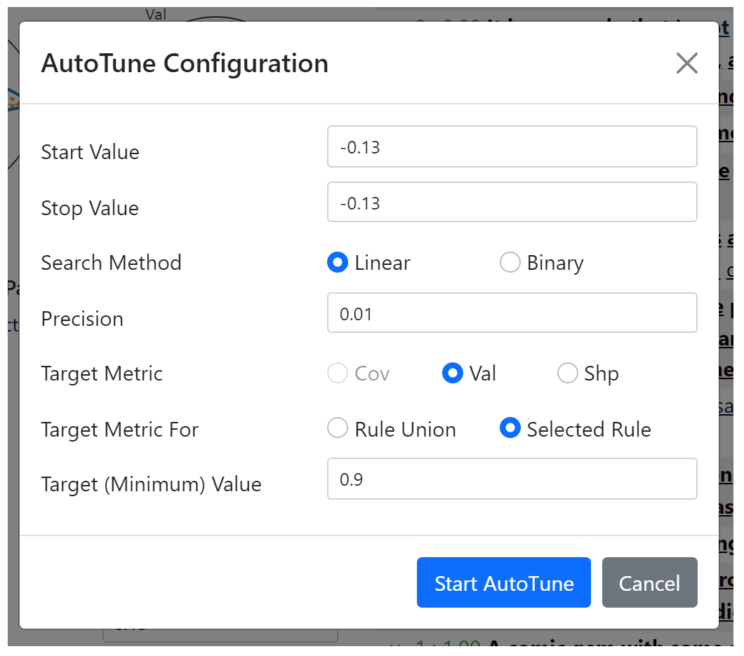 The objective of the search is specified by the triplet of (target metric, target metric for, target value). For example, in the pop-up above, the search tries to find a parameter value that achieves a validity value of at least 0.9 for the selected rule. Note that the coverage metric is not available for selection since we are tuning a parameter for the behavior function. All three metrics can be selected for parameters of the applicability function.
There are two available search methods, linear search and binary search. Both methods try to find a satisfying value between the start value and the stop value. The start value and stop value are initialized to the current parameter value, but they should be changed appropriately.
The linear search uses precision as a step size. Suppose that we have start value = 0.0, stop value = -1.0, precision = 0.01. Then it sequentially evaluates values of 0.0, -0.01, -0.02, ..., -0.99, -1.0, and terminates when the objective is first met. Thus, it stops at the satisfying value closest to the start value.
The binary search uses precision as the smallest halving length. It requires that the stop value is feasible (i.e. satisfies the objective), and initializes the interval [left, right] to [start value, stop value]. At every iteration, if the mid-point of the interval is feasible, it uses the interval [left, mid-point] as the new interval, and if it is infeasible, it uses [mid-point, right]. The procedure stops when the interval length is smaller than precision. Thus, if the metric value is monotonically increasing in the direction of start value to stop value, then the binary search will also output the satisfying value closest to the start value, but can be much faster than the linear search. However, with non-monotonicity, it could miss the closest satisfying value, which may be undesirable.
When the search is successful, the parameter value is updated. When it is not, the parameter value remains the same, and an error message banner alerts the user of the failure.

Panel E

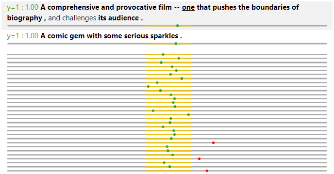
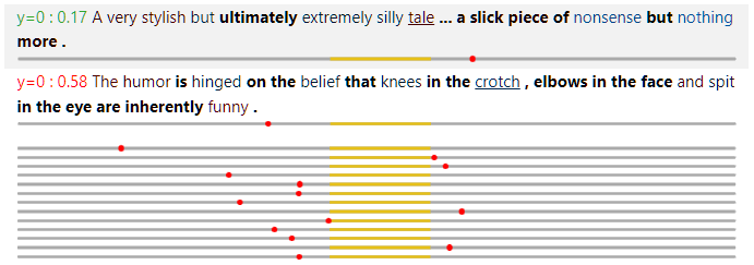
This panel visualizes the rules and rule union on specific data instances. On top are three control buttons.

• The first button toggles between visualizing the whole rule union and visualizing only the selected rule.
• The second button toggles between visualizing the entire sentence or only one FEU within the sentence.
• The last button shuffles the data and presents a new batch of instances. A random seed for the shuffling is used, so batch sequences are the same for multiple exsum runs.

The syntax highlighting on each word conveys additional information.

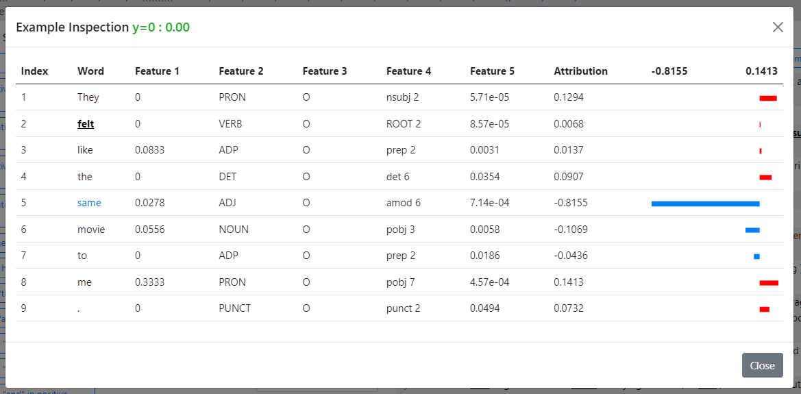
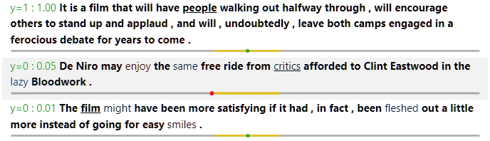
• The ground truth and model prediction (in probability for the positive label) is shown at the beginning, on the left and right of the colon respectively. When the prediction is correct (using 0.5 as the threshold), the text is in green. Otherwise, the text is in red.
• An underline under a word means that it is covered (by the selected rule or the rule union, depending on toggled value in the first button).
• For a covered word, the bold font means that it is valid according to the behavior function, and the normal font means that it is invalid.
• The color on each word represents its attribution value, with the value of 1.0 rendered in full red, and value of -1.0 rendered in full blue. Thus, to effectively use this functionality, it is recommended that attribution values are normalized to have maximum magnitude of 1.0.
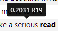
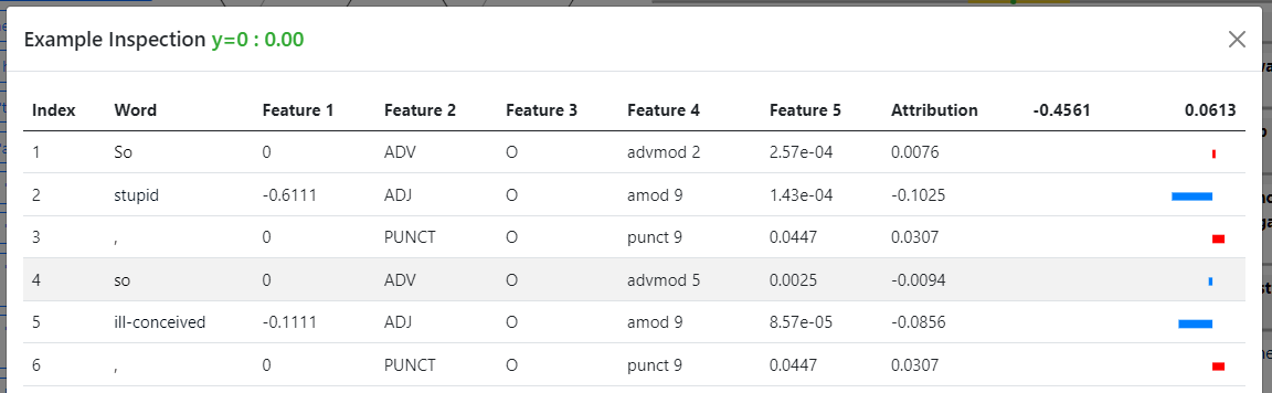
• Hovering the mouse on each word reveals a tooltip showing the numeric attribution value and the rule (if any) that covers this word. An example is shown in the image below (in this case, Rule 19 is invalid on the word "serious" because the word is not in bold font).
  

In addition, clicking on each sentence opens up a pop-up of detailed information of the sentence. The major addition is the table of feature values for each word. An example is shown below. The last column also shows the attribution value for each word in a bar chart. When the second button is toggled to the FEU mode, a random applicable word (FEU) is selected, and it is underlined. Its behavior function output is plotted along with its actual attribution value. In the image below, the whole gray bar represents attribution values from -1.0 to 1.0. The yellow bar represents the behavior function output. The dot represents the attribution value of the word, with green for a valid prediction by the behavior function and red for an invalid prediction. Againt, because the range of [-1.0, 1.0] is used, the attribution values should be normalized to within this range for correct rendering. One issue with the FEU mode is that the information density is much lower, as row of the visualization can only be used to visualize one word. Thus, to give a sense of how well the behavior function performs overall (e.g. is it too narrow, too wide, or even improperly skewed), additional FEUs are visualized with the bar graphics only at the end, as shown in the image below. The sentence and FEU corresponding to each bar can be inspected in the same pop-up table by clicking on the bar, where the FEU has its row highlighted, as shown in the image below (the FEU is the fourth word "so"). Finally, the user can also hide all valid FEUs and just focus on invalid ones, using a button that appears in this mode, as shown in the image below. The effect of toggling this button is shown in the image below.

Development Manual [Back to Top]

It is strongly recommended to read the paper first, in order to understand the high-level ideas and goals of the package.

Class Structure

The diagram below describes the has-a relationship among classes as a tree, where parent nodes contain child nodes. All classes are under the package namespace exsum (e.g. the fully quantified class name for Model is exsum.Model). The three green classes represent list membership. For example, a Rule has a list of Parameters. For the BehaviorRange shown in yellow, it is technically not contained in Rule, but is instead produced by its behavior function. We include it here for completeness. The top-level Model object is passed to the command exsum to start the GUI visualization.

Class Documentation

‣ class Model

The Model class is the top-level object that contains everything necessary about the rule union and the dataset on which the rule union is evaluated. It should be initialized as:

model = Model(rule_union, data)

where rule_union and data are objects of the RuleUnion and Data class respectively. The Model class is also responsible for calculating metric values and producing instance visualizations (which are queried by the GUI server), but users should not be concerned about these functionalities.

‣ class RuleUnion

A RuleUnion is specified by a list of rules and a composition structure of these rules. It should be initialized as:

rule_union = RuleUnion(rules, composition_structure)

• rules is a list of Rule objects. As described below, each rule has an index, which we assume to be unique.
• composition_structure specifies how the rules are composed. If a rule union contains only one rule, it is an integer with value being the rule index. Otherwise, it is a tuple of three items. The first and the third one recursively represents the two constituent rule (specified by an integer) or rule union (specified by a tuple), and the second one is either '>' for precedence mode composition, or '&' for intersection mode composition.
  For example, the composition structure of (3, '>', (1, '&', 2)) means that rule 1 and 2 are first combined in intersection mode, and then combined with rule 3 with a lower precedence.
  Not every rule needs to be used in the composition_structure, but no rule can be used more than once.

The RuleUnion class is also responsible for supplying the metric values requested by the Model and generating the counterfactual RuleUnion without a specified rule, but users should not be concerned about these functionalities.

‣ class Rule

A Rule contains the following information: index (an integer), name (a string), applicability function a_func and its parameters a_params, and behavior function b_func and its parameters b_params. It should be initialized as:

rule = Rule([index, name, a_func, a_params, b_func, b_params])

Note that the constructor takes in the single variable of a list that contains every piece of information rather than each piece separately. a_func and b_func are native Python functions. They have the same input format: an FEU as the first input, followed by a list of current values for the parameters, as below for an example of an applicability function with three parameters:

def a_func(feu, param_vals):
    param1_val, param2_val, param3_val = param_vals
    ...

a_func returns True or False to represent the applicability status of the input FEU, and b_func returns a BehaviorRange object to represent the prescribed behavior value.
Sometimes a_func and b_func share many common implementation details. In this case, it could be more convenient to combine them into one ab_func. In this case, the rule can be initialized as

rule = Rule([index, name, ab_func, a_params, b_params])

Note that again a list is provided, but this time with five items instead of six. The Rule constructor uses the length of the list to distinguish between these two cases. ab_func should take in the FEU, a list of current values for a_params and a list of current values for b_params, and return a tuple of two values, True or False and a BehaviorRange object, as below:

def ab_func(feu, a_param_vals, b_param_vals)

When b_func or ab_func is called for a non-applicable input, arbitrary object can be returned (but the function should not raise an exception) and the result is guaranteed to not be used. Furthermore, the name of the rule has no effect on everything else, and is only for human readability.

‣ class Parameter

We assume all parameters take floating point values. A Parameter object encapsulates everything about a parameter, including its name, value range, default value and current value. It is initialized as

param = Parameter(name, param_range, default_value)

where name is a string, param_range is a ParameterRange object, and default_value is a floating point value. The current value is set to the default_value on initialization and reverted back to it whenever the user presses a Reset button on the GUI.

‣ class ParameterRange

We assume that all parameter value ranges are continuous intervals, so a ParameterRange is specified by its lower and upper bound:

param_range = ParameterRange(lo, hi)

where lo and hi are floating point values for the two bounds. Note that the interval is assumed to be a closed interval. To represent an open interval, offset the bound value by a small epsilon value (e.g. 1e-5).

‣ class BehaviorRange

Similar to ParameterRange, BehaviorRange objects are also defined as closed intervals. However, a key difference is that a BehaviorRange allows multiple disjoint intervals. For example to represent that an attribution value should have extreme values on either side, the behavior range could be [-1.0, -0.9] ∪ [0.9, 1.0]. Thus, it is initialized as

behavior_range = BehaviorRange(intervals)

where intervals is a list of (lo, hi) tuples. In the case where a single closed interval is needed, an alternative class method is also provided in a way similar to the syntax of ParameterRange:

behavior_range = BehaviorRange.simple_interval(lo, hi)

To represent an open interval, offset the bound value by a small epsilon value (e.g. 1e-5).

‣ class Data

A Data object represents the set of instances along with their explanation values, on which the rules and rule union are evaluated. The main data are stored in a SentenceGroupedFEU object. In addition, to compute the sharpness metric, the probability measure for the marginal distribution of all explanation values need to be used. Operations on the probability measure is enabled by the Measure object. With these two objects, a Data object can be initialized as:

data = Data(sentence_grouped_feu, measure, normalize)

where normalize is an optional boolean variable (default to False) that specifies whether the explanation values should be scaled so that all are within the range of [-1.0, 1.0].
If normalization is enabled, first the maximum magnitude of all explanation values (positive or negative) is found. Then all explanation values are divided by this magnitude, effectively shrinking (or expanding) them around 0, so that the maximum magnitude is 1.0. The Measure object is also scaled accordingly. Its default value is set to False to prevent any unintended effects, but we recommend normalization (or pre-normalization of explanation values before loading into this Data object) since the coloring used by the GUI text rendering assumes -1.0 and 1.0 as the extreme values.

‣ class SentenceGroupedFEU

Recall that for NLP feature attribution explanations, an FEU is word contexualized in the whole input. Storing an entire copy of this information for every word in a sentence is wasteful. So the SentenceGroupedFEU class is designed to represent a data instance with its explanation as a whole. A data instance contains the following information:

• Ground truth label, assumed to be binary,
• Model's predicted probability of the positive class (floating point in [0, 1]),
• A list of tokenized words in the sentence,
• A list of features, one for each word represented as a tuple. The number of features for each word should be fixed. These features are used by the a_func and b_func rather than the classifier, and thus should be human-interpretable, and
• A list of floating point attribution values, one or each word.

It should be initialized as:

sentence_grouped_feu = SentenceGroupedFEU(words, features, explanations, true_label, prediction)

where words is a list of strings, features is a list of tuples (of arbitrary elements), explanations is a list of floats, true_label is either 0 or 1, and prediction is a float between 0 and 1. The items in words, features and explanations should be aligned with each other, and thus the three lists should have the same length. A SentenceGroupedFEU in spirit contains a list of FEUs. However, to save space, this list is never explicitly kept, but elements of it are generated on the fly. Users should not be concerned with the details.

‣ class FEU

As seen above, the construction of a SentenceGroupedFEU does not require the actual instantiation of FEUs. However, as a_func and b_func take inputs of this class, it is important to familiar with its instance variables. An FEU object feu has the following instance variables:

• feu.context points to the SentenceGroupedFEU object from which this feu is created;
• feu.idx is an integer for the (0-based) position of the FEU in the sentence;
• feu.word is a string for the word of the FEU;
• feu.explanation is a float for the explanation of the FEU;
• feu.true_label is an integer of either 0 or 1 for the ground truth label;
• feu.prediction is a float in [0, 1] for the model's predicted probability for the positive class; and
• feu.L is an integer for the length of the whole sentence.

Technically, all instance variables beyond the first two are syntatic sugars, as they can be retrieved from the parent SentenceGroupedFEU. However, they are included for convenience due to frequent use.

‣ class Measure

The Measure class represents an estimated probabilty measure on the marginal distribution of explanation values. It is computed by kernel density estimation, and the resulting cumulative distribution function is approximated by a dense linear interpolation for fast inference. This is a relatively expensive computation, especially for a large dataset. Thus, it should be pre-computed and provided explicitly when constructing the Data object.
It should be initialized as:

measure = Measure(explanations, weights, zero_discrete)

• explanations is a flattened list of all explanation values for all data instances;
• weights is a flattened list of the (unnormalized) weights corresponding to the items in explanations. ExSum defines metric values by considering each data instance as equally weighted. Thus, an FEU in a longer input receives less weight than an FEU in a shorter input. The simplest way is to assign 1 / feu.L as the weight for the explanation; and
• zero_discrete specifies whether the zero explanation value should be considered as a point mass in the probability distribution (i.e. a mixed discrete/continuous distribution). Some explainers (such as LIME with LASSO regularization) produce sparse explanations where a large fraction of explanation values are strictly 0. This case should be modeled with zero_discrete = True, while generally continuous distributions should be modeled with zero_discrete = False.